Understanding PID Controllers

This post takes a look at the PID Controller, which is widely used in robotics for providing more accurate motions of any moving parts on a robot. We will go through some basic control theory to give a better understanding of what a PID controller is, then look at each of the P, I, and D terms to develop a more intuitive understanding of the controller. From there, you should be able to use the controller in your own projects.
If you're interested in seeing this post in video form, check the YouTube link below:
What is PID Control?
The PID in PID control stands for Proportional Integral Derivative. It is a way for robots to control their movements to be smooth and accurate, which helps them carry out their tasks correctly. For example, PID control can help a robot arm move to pick up an object without hitting into it or missing it entirely. Another example is moving wheels at the requested speed to make navigation more accurate.
PID control is used in many different fields, not just in robotics, but this post focuses on the use of PID control in robotics.
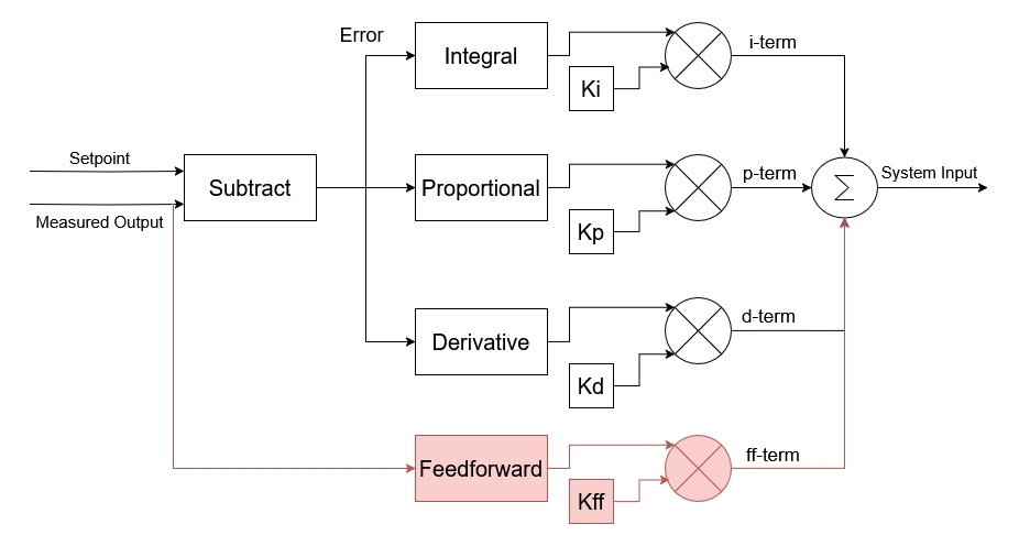
To explain more about what PID control is and how it works, including the general overview from the diagram above, it helps to define a few terms from control theory.
Control Theory Terminology
First, any kind of control is the process of adjusting an output to be at a required level, or setpoint. This could be the heat level of a tank of water, which can be controlled by burning gas to heat the water. Another type of control is controlling the speed of a motor to spin a wheel or move a robot arm's joint.
A controller is a process responsible for controlling the output. In cars, the controller is a human, and the control process is to reach and maintain a certain speed by changing the acceleration of the car with an accelerator pedal. The controller should also respond to changes in speed as quickly as it can; if the desired speed increases, the controller should accelerate to the new setpoint, then maintain the speed there. Controllers should try to reach the setpoint quickly without overshooting or oscillating about the setpoint.
The controller produces a system input, which is the signal it uses to adjust the system. In a car, the system input is the accelerator position. In turn, the system response or system output is how the system behaves based on the system input; in a car, the system response is to speed up. Finally, the measured output is the measured value of the system response, such as the reading on a speedometer.

Open and Closed Loop Controllers
Controllers can either be open loop or closed loop, depending on whether they measure and react to the system as part of the control process.
Open loop controllers do not react to the measured output as part of the control process. Instead, the controller guesses the correct system input to reach the setpoint and assumes the system responds as expected. For example, it tells two motors to move at a particular speed and assumes that they move at exactly that speed, with no issues. This control works well enough in many applications, and it's the type of control we used for the JetBot.

Closed loop controllers use measured output from the system to adjust the system input for better control. With a differential mobile robot, the controller can use wheel encoders to measure how fast the motors are actually moving, then adjust how fast it tells the motors to move to correct for the change. This allows the robot to keep a constant speed even if one motor is slightly more powerful than the other one.
PID Controller
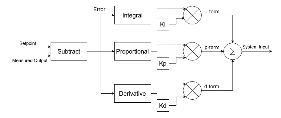
With our control theory terms defined, we can now define PID control as a form of closed loop control that calculates its system input from proportional, integral, and derivative terms based on the measured output. The controller first calculates the error term as the difference between the setpoint and the measured output, then uses the error to form the control terms:
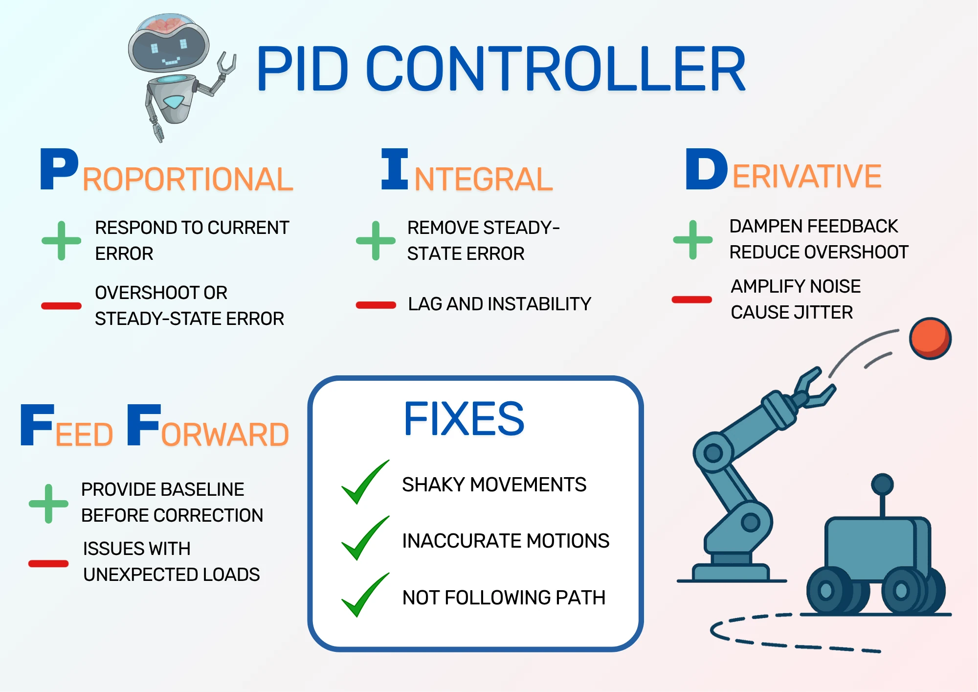
- Proportional (P): the error is directly multiplied by a constant Kp to get the proportional term (p-term).
- Integral (I): tracks the total error over time, and multiplies this value by a constant Ki to get the integral term (i-term).
- Derivative (D): calculates the change in error by comparing to the previous error, then multiplies this value by a constant Kd to get the derivative term (d-term).
The controller adds these values together to form the system input.
The parameters Kp, Ki, and Kd are the tuning parameters of the controller. These three values alone determine how a controller reacts to the measured input, so adjusting a controller to work for a system (tuning the controller) is the process of finding the parameters that get the most reliable output. This is generally done manually by running the system and adjusting parameters to get the best response from the controller.
Why use a PID Controller?
A huge advantage of using a PID controller is that it can be used for any system. Instead of modelling a system and building a controller that works only for that system, PID controllers are versatile enough to work for that system out of the box, even if they don't work quite as well as another controller. As they work very well in most applications, they are widely used in robotics.
PID controllers are therefore used for controlling most moving parts on a robot. When the performance of a robot depends on how well it responds to input commands, PID controllers can help improve that performance, making the robot move along desired paths much more closely or reach for an object more accurately. Some parts don't need PID controllers, or don't have the sensors necessary to provide feedback data; still, PID controllers are very commonly used, so it's worth understanding how they work.
Understanding PID Controllers
So far, we've discussed what a PID controller is, and why we use them - particularly in robotics. Now, to give a more intuitive understanding of how they work, we will look at an example, then look at each of the P, I, and D terms in turn to see the effect they have on the system input.
Driving a Car
Let's take the example of a car with a human driver. The driver has one pedal to accelerate or brake the car; pushing the pedal further down accelerates more, and releasing the pedal slows the car down. The task of the driver is to keep the car at a steady speed in spite of winds, changes in the road, and so on. The driver should also speed up the car or slow it down to turn corners, drive through towns, or any other changes needed.
We're going to make the driver's job more difficult by saying that the pedal is stiff. Releasing the pedal means it slowly brakes, and pressing the pedal takes time because of its stiffness.
The driver is driving through a town at 50 kph and will soon leave the town. Once back on the main road, the driver plans to accelerate up to 90 kph. How should the driver do it?
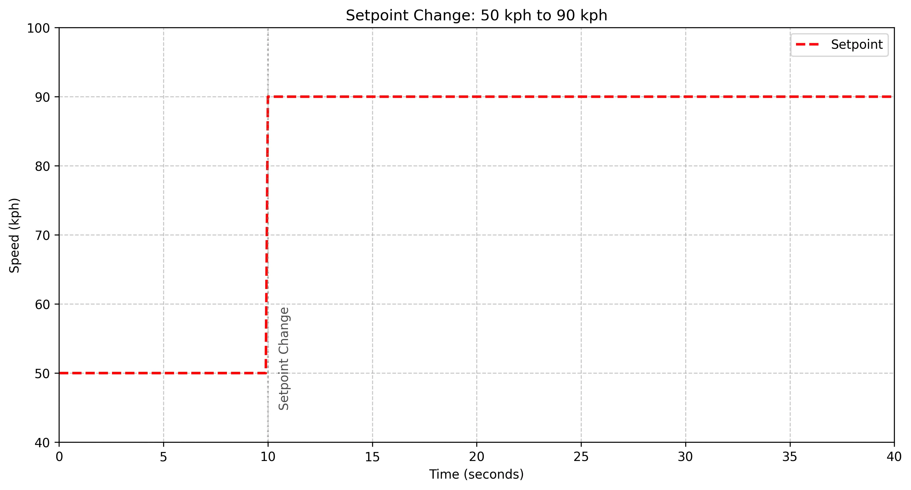
The simple solution is to push the pedal hard to accelerate the car, then mostly release the pedal to maintain the correct speed. However, because the pedal is stiff, the car keeps accelerating. The car has now overshot its target speed.
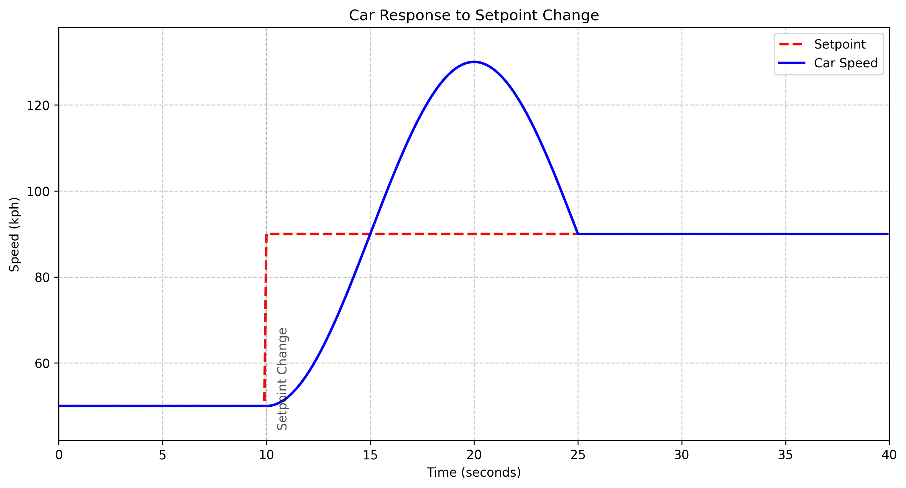
The driver decides to try a different method: releasing the pedal based on how close to the target speed the car is. This is a P controller (it only contains the P component of the PID controller), as it relies on multiplying the error between the current speed and the set speed. As the car gets closer to the target speed, the error reduces, so the driver releases the accelerator a bit more.
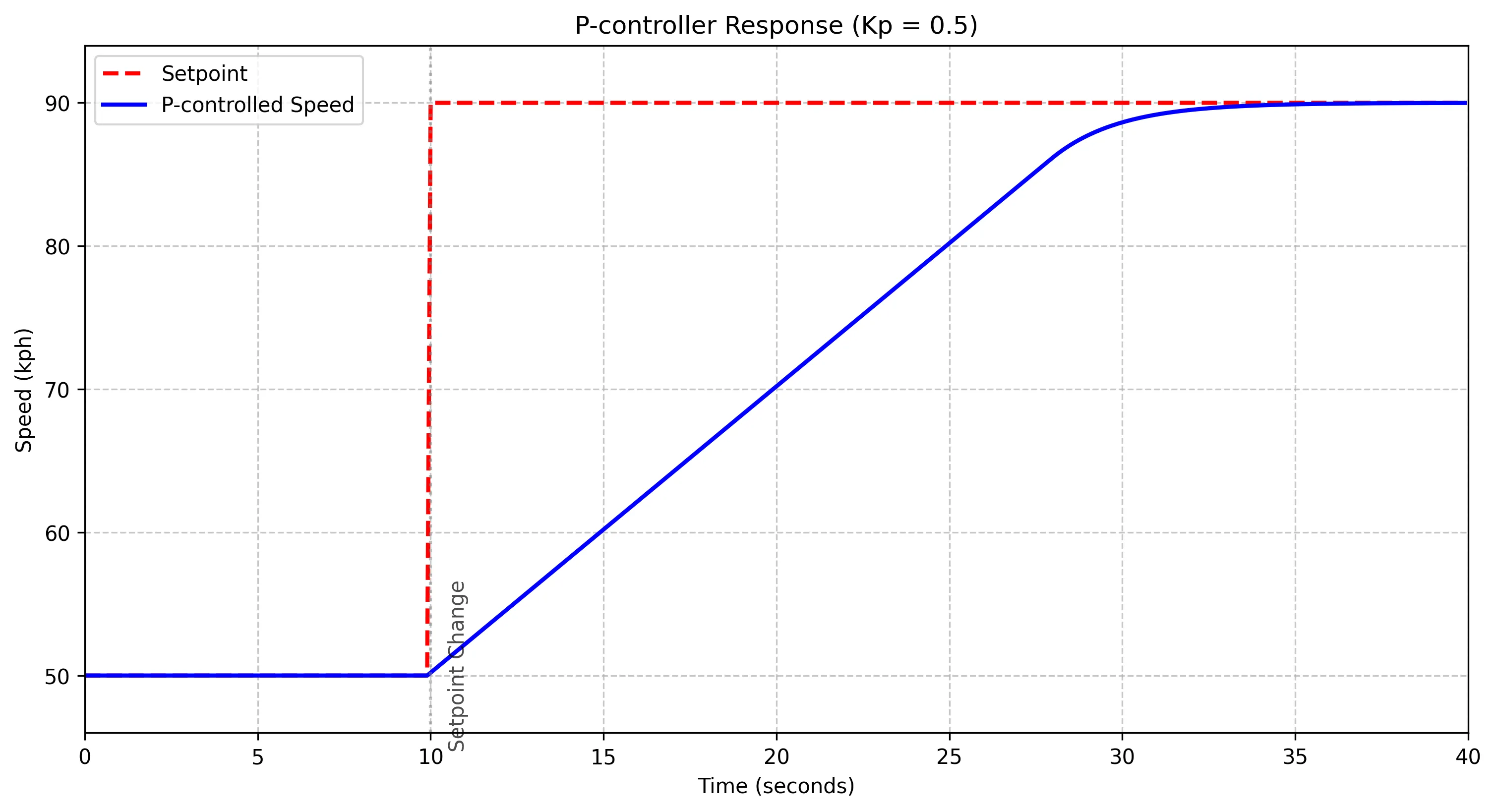
We can see that the car took longer to reach the target speed, but didn't overshoot at all. This is better behaviour for our system, but we could try different Kp values to reach the target speed faster. The best value depends on how the system responds, which is in this is largely defined by how stiff the accelerator pedal is and how fast the car can accelerate.
PID Visualisation Tool
The car example is pretty simple, but already needs a closed loop controller. To better show how the different PID terms work, I've built the interactive tool below. (Cursor saved me a lot of time building it - thanks, Cursor!)
The tool shows how a robot arm joint behaves with different PID control parameters. The measured output is the robot joint velocity, and the system input is a desired velocity. However, because the robot arm joint has to move the arm and possibly a payload, it has to accelerate to the requested velocity. This is similar to the car's accelerator pedal being stiff, and causes a lot of oscillation.
The tool is available below. Feel free to play with the sliders for all of the PID components, but these will be discussed in more detail later in the article. The time slider shows the values of the system at any point in time along the system response, including the current integral value (highlighting the relevant area) and the current derivative value (shown as a purple tangent to the line).
Proportional Term
The first term to look at is the proportional term. This is a multiplication of the error, so it's the simplest to calculate - and to understand! Decreasing Kp will move the system response down and to the right, while increasing it moves it up and to the left. Too large, and the system starts to oscillate.
For this system, the oscillation happens for any amount of Kp. Try moving the Kp value from the very bottom to the very top, and see what happens.
P controllers can work in isolation, depending on the system. It is also possible to add only the I term, only the D term, or both I and D terms.
- P + I: PI controller
- P + D: PD controller
- P + I + D: PID controller
Let's look at adding the derivative term to our controller.
Derivative Term
Our controller will now adjust the system input based on the rate of change of the error. This means that at each point in time, the current error is subtracted from the previous error and multiplied by Kd, the derivative constant. Our controller is now a PD controller.
Adding a derivative term effectively dampens the response, meaning that the output can't change as quickly. Take a look at moving the D-term until the system has a smooth ramp up, then flattens out. You should see that the gradient of the line changes as you move the time slider, shown by a purple line. This shows the gradient that is being multiplied by Kd.
I get a good response and no overshooting with Kp=1.80, Kd=0.90.
You should see that the output is getting closer to the setpoint line. This is exactly the behaviour we want! In general, the d-term helps to dampen the system response to make it more stable, but tends be more sensitive to noise. Imagine your sensor is noisy and suddenly produces a false high value; the controller would give a very large response to the large gradient from the false reading.
Still, the system response is not that close to the setpoint. There is a gap between the line and the set point, which we call a steady-state error, and can be corrected using the last component of the PID Controller: the I-term.
Integral Term
For the integral term, the error is added up over time. This is a process called integration, and for our controller it means adding the error to a running total, then using that total error to adjust our system input. The larger the error, or the more time the error exists for, the larger the total error will grow, and the more effort the controller puts in to reach the setpoint. This helps compensate for steady-state errors over time.
Just as with the other terms, we then multiply by a constant, Ki in this case, and add it to the total output of our controller. Increasing Ki to be too large can lead to oscillation and overshooting, but if it's small enough, it can compensate for errors over time and bring the output to the right setpoint.
Try adjusting Ki in the tool below and see the effect on the output for very large and very small values. Then try to match the setpoint as closely as possible, including adjusting the Kp and Kd parameters. As you move the time slider along, you should see the area between the system response and the setpoint highlighted; this is added to the total error over time. You can also see the integral value, which is the total value at that point in time.
I get a good response by using Kp=1.80, Ki=1.20, and Kd=0.90.
Feedforward
Our controller is looking pretty good! It doesn't exactly meet the setpoint when it changes, but in reality, it's not possible for a system to exactly match the setpoint like that. There will always be some delay, and likely some ramping to meet the setpoint. This is true of robots as much as other systems.
Our final (optional) parameter to tune is feedforward. This isn't necessarily a part of PID controllers in general, but it is available in the ros2_control implementation of a PID controller. That's why I haven't mentioned it until now.
The feedforward parameter Kff is multiplied by the input value, not the error value. This provides an initial value for the controller that it can change on top of, which means the P and I parameters don't need to work as hard to correct for error.
Try modifying the constant Kff in the tool to see the change in output. If you can, get a system response even closer to the setpoint.
The best response I can get is using Kp=5.00, Ki=0.00, Kd=1.30, and Kff=0.50. This means we no longer need the i-term, which makes the controller simpler, and it should be more stable.
With our controller tuned, you can now play with the sliders again to see what effect each slider has on the system response. This helps build intuition about how the different parameters work for the controller.
PID Controllers with ROS 2
With our understanding of PID controllers, the next question is how to implement one for a robot. One way to do so is to use the pre-built PID controller from ros2_control.
The PID Controller can be launched as part of a ros2_control system, and tuned by parameters in the configuration file. The controller documentation has recommendations on whether to use PI, PID, or PD controller based on the measured output and the system input types. It also provides an example project showing how to use PID controllers with a differential mobile robot. In a future post or video, I plan to go through this example more thoroughly, showing how to set up and tune the two PID controllers used to control each wheel on a real robot.
Summary
In this post, we took a look at PID control, which is a fundamental concept in robotics for achieving precise, responsive motion. It's a type of closed loop control that continuously adjusts a system's input based on the error between the measured output and the desired output. This error is used by the p-term, integrated for the i-term, and subtracted from the previous error value for the d-term, with each term multipled by a parameter Kp, Ki, and Kd respectively.
We saw the need for a closed-loop controller with a car driving example, then looked at each term of the PID controller to see its effect on the system input, using an interactive visualisation of a robot arm joint model with payload to do so. We also looked at feedforward control as used in ROS 2's implementation, and finally discussed how to implement a PID controller for real using ros2_control.
Having an intuitive understanding of PID controllers will help make your robots more accurate, stable, and effective. If you have a real robot with a feedback mechanism, see if you can use PID control to make the movement smoother and more effective. This is exactly what I hope to do in a future post!